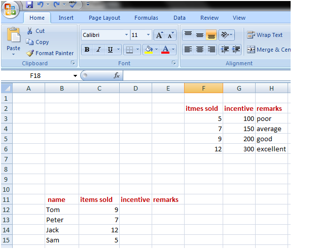
Excel Vlookup

Vlookup is an advanced Excel function that helps extract values from the database. Vlookup can filter large volume of data to provide the appropriate values based on the given conditions.

V lookup can be used in two ways, to find an exact match and to find the closest match. In this example, it is used to find an exact match.

Using Vlookup to find an Exact Match:

In this example, A company wants to know the incentive and remark for each employee. Vlookup is used to filter the database and extract correct incentive and remarks for the employees.

See the image given below, one table is showing the incentive and remarks for the number of items sold. Second table is created by the company to display the extracted figures; incentive and remarks for the employee.

Using vlookup, on entering the number of items sold by an employee in column C, the Excel automatically fills the corresponding incentive figure and remark for the employee.

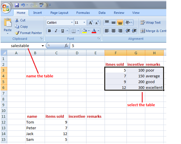
Before applying the vlookup, select the data table excluding the headings and name it in the name box, like we named it “salestable” in this example. See the image given below:

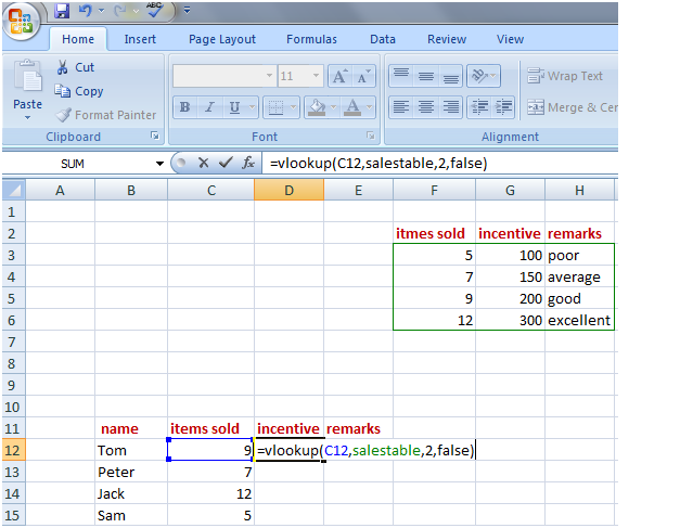
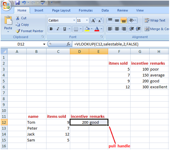
Now we will use vlookup to retrieve the correct incentive and remark for Tom.

Type the vlookup function in the cell where you want to display the incentive. D12 is the cell in this example, where we want to display the incentive for Tom.

• In the cell D12 type: =vlookup(
• Now type what you want to find or look for in the data table. In this example, it is the value of cell C12, so type: C12,
• Type the name of the data table containing the information and a comma: salestable,
• Type the column number, the column of data table from where you want to retrieve the information then type a comma. In this example, it is second column of data table so type: 2,
• Now type “false” which tells excel to retrieve the information for exactly the same value that is in cell C12, not anything else close to it. In this example, it will retrieve information for 9 items sold from the second column of data table. So, if figure 9 is not available in data table it will display an error.
• Close the bracket and press the Enter key. You will get the incentive for Tom.

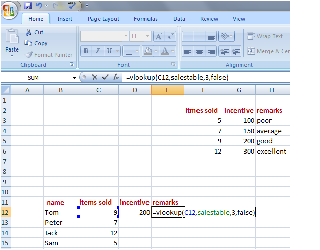
Now to retrieve the remark for Tom, type the same function in cell E12, but select the third column of data table instead of second as remarks for employees are given in the third column of the data table. After getting the remark for Tom using fill handle you can get the incentive and remarks for other employees. See the images given below:

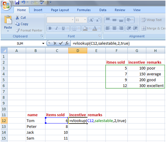
Using Vlookup to Find Closest Match

In the previous example, vlookup is used to find an exact match. But what if Tom sells 6 items then how we retrieve information from the data table. In this case, we will use vlookup to find the closest match for our lookup value.

For that we will type “true” instead of “false” in the formula. It tells Excel to find the closest match for the vlookup value if it doesn’t find an exact match in the data table.

Vlookup always looks for smallest closest match available in the data table so in this case for 6 items sold by Tom it will find the incentive for 5 items sold as it is the lowest closest match for 6 items sold. So it will retrieve incentive 100 from the second column of the data table.

See the example:

Items sold by the employees are not matching with the data table. So “true” is used in the formula to find the closest match for the number of items sold by the employees.

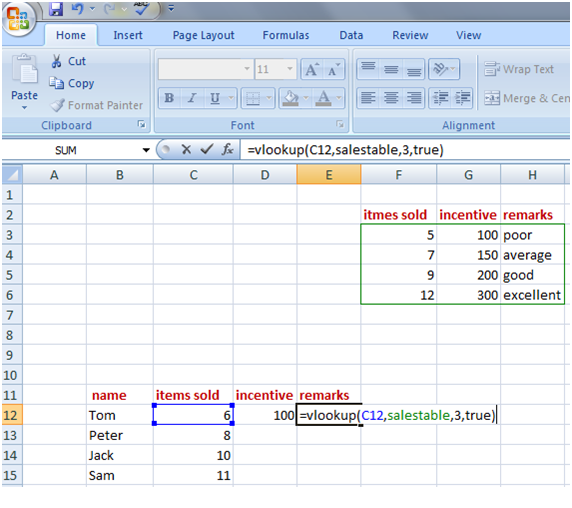
Again to find the remarks for the employees “true” is used instead of “false” in the formula. See the image given below.

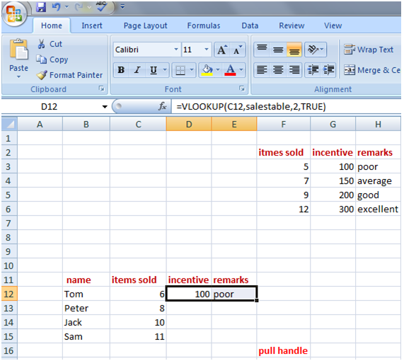
After getting the details for Tom use fill handle and get the details of other employees.

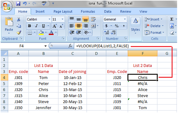
Using Vlookup to Match Lists

Vlookup can be used to match lists, to see if the lists are matching or there are some missing values. In this example, we use vlookup to retrieve the name of employees to list 2 from list 1 data. See the image given below:

The vlookup function is: =vlookup(E4,List1,2,false)

• In this function we have named the list1 data table as “List1”.
• E4 is the cell which we want to look for in the “List1”.
• “2” is the second column of list1 from where we want to retrieve the information.
• “False” is used as we are looking for an exact match.

Vlookup displays “#N/A error code” for the employee codes of list 2 that are not available in list 1 data.